Chapter 11 Discrete Random Variables
This chapter marks the start of our introduction to probability, the math that allows us to characterize chance and uncertainty. For the math-phobic or just math-rusty, the next 3-4 chapters will likely be your least favorite topics in this course. Nevertheless, we need to understand probability in order to understand sampling distributions, which are the foundation for statistical inference.
11.1 Uncertainty \(\ne\) Equally Likely Outcomes
Suppose you’re planning a vacation trip to a beautiful beach. While talking to your aunt on the phone, she exclaims that she’d never go there. She saw a story where someone was attacked by a shark. She admits that it’s not certain that you’ll be attacked by a shark as well. However, she argues, you either will be attacked or you won’t be; and, because you just never know, the likelihood is 50-50 that you’ll be attacked. You plan on spending a week at this idyllic beach, but don’t relish the thought of being attacked on at least three of those days.
Your aunt’s version of probability equates uncertainty with all outcomes being equally likely. This line of thinking is something along the lines of: we can’t know for sure what will happen, therefore each of the possible outcomes is equally likely. However, if we spend only a few seconds thinking about our daily lives, we know this is not the case. When I walk outside, I might be hit by a bus or not. I don’t know what will happen on any given day, but I at least have the sense that being hit by a bus is highly unlikely – it’s certainly not a 50-50 chance.
The same goes for driving to work in the morning or whether my home will catch fire and burn down. In fact, the insurance industry is based on calculated risks (i.e., probabilities) – for example, that their clients will have an auto accident, experience a fire that burns down part of their house, or die. These probabilities are based on factors such as a person’s (or car’s) age and, among other things, evidence of risky behavior like smoking or racking up speeding tickets. Although it is unknown on any given day whether a person will experience an auto accident, a home fire, or die, the likelihood is usually very very small – not 50-50. Moreover, depending on the background factors (e.g., age, risky behavior), insurance companies can adjust their estimates for each person. That’s how they make money! If your aunt would like an even more extreme example, just consider casinos… they set the probabilities of winning for each game. Those probabilities are usually not 50-50!
As one last example, suppose the weather forecast tells us that the chance of rain today is 10%. It might rain or it might not. We don’t however conclude that the chance of rain is 50-50. Rather, we conclude that it’s unlikely that it will rain, but there’s some small chance. To the best of the forecaster’s knowledge, on days like today, it rains 10% of the time and doesn’t rain 90% of the time.
The point here is that uncertainty only implies that we don’t know for sure what will happen. However, probability distributions sometimes give us precise information about what is likely to happen.
11.2 Variables, Variables, and Random Variables
In a course like this, the term “variable” gets thrown around a lot. We began the course talking about R and different variables there. In R, a variable is an object to which we assign something: a number, a vector of numbers, TRUE or FALSE, a string, etc. Technically, it is the name of a storage location that we can refer to by a useful name that we create, especially when we want to refer to that object multiple times.
In the sections on variables, operationalization, and measurement, as well as that on descriptive statistics, we referred to variables and their scale and to the operations we could perform with them. In that role, the variable represented an existing vector of data (a sample) for which we might calculate the mean or median.
Random variables are quite different. A random variable (RV) is a mathematical construct. We assume that there is some experiment or event at which point we realize, sample, draw, or simply observe a value from a probabilistic process. Suppose we’re going to flip a coin. Ahead of time, we don’t know whether it will land Heads or Tails. The flipping of the coin is the realization, sampling, or observation of the result. We finally see the outcome: Heads or Tails. Importantly, although we don’t know the outcome before the experiment, sampling, or observation, we’ll assume that we know the possible outcomes that the random variable can take and that we know which of those outcomes are more likely to occur. We’ll make this more explicit later.
For now, the important part is understanding that a random variable is conceptually different from the variables we see in an R dataset. A variable in an R dataset is an existing sample – a set of observations. A random variable is a mathematical construct that helps us describe a probabilistic process where we have not yet observed the outcome. That’s not to say that random variables and our sample variables aren’t related. They are and we’ll talk more about that later.
Consider the following random variables:
Flipping a coin
Rolling a die
Number of auto accidents in the US in a year
The winner’s vote share in an election
The first three are discrete random variables. They are either categorical (flipping a coin) or interval variables that are finite (rolling a die) or countably infinite (number of auto accidents per year). The last variable is a continuous random variable, since we treat the vote share (proportion) as being able to take any value between 0 and 1. Continuous random variables have slightly different rules than discrete random variables. We’ll focus on discrete random variables here and turn to continuous random variables in Chapter 13.
11.3 Discrete Random Variables
For a discrete random variable \(X\), we need to specify
The possible outcomes (or event space) for \(X\).
The probability that each of those outcomes occurs.
The following are examples of the possible outcomes for different random variables:
Flipping a coin: \(Y \in \{ H, T \}\)
Rolling a die: \(Y \in \{ 1, 2, 3, 4, 5, 6 \}\)
Auto accidents this year: \(Y \in \{ 0, 1, 2, 3, 4, \ldots \}\)
Generally: \(Y \in \{ y_1, y_2, \ldots, y_k \}\)
The \(\in\) symbol should be read as “is an element of”. The coin flip example would therefore be read as: “The random variable \(Y\) is an element of \(\{ H, T \}\),” where H(eads) and T(ails) are the possible outcomes. Notice that the coin flip and die toss have finite sets of outcomes. The number of auto accidents is countably infinite.
For a given random variable \(Y\), we also need to specify the probability for each possible outcome. Let’s consider the first two random variables above. For a fair coin flip, we can write the probability mass function (PMF) as
\[\begin{equation}
\Pr(Y=y) = \Pr(y)= \left\{ \begin{array}{ccl} .5 & \, & \mbox{if }\, y=H \\ .5 && \mbox{if } \, y=T \end{array} \right.
\tag{11.1}
\end{equation}\]
There are a few things packed in here. First, I’ll tend to use the terms “probability mass function” and “probability distribution” interchangeably for discrete random variables. We’ll see later that it’s a little more complicated when we get to continuous variables. Second, we’ll typically use an uppercase \(Y\) to refer to the random variable and a lowercase \(y\) to refer to a value it might take. Although I have written out \(\Pr(Y=y)\) to refer ot the probability that random variable \(Y\) takes the value \(y\), I’ll usually use the shorthand \(\Pr(y)\) to refer to the same thing, where the \(Y=\) is implied. Notice that the PMF above specifies both (1) the possible outcomes \(\{H, T\}\) and (2) the probability of observing outcome.
Turning to the die toss, assuming the die is fair, we can write its probability mass function as \[\begin{equation} \Pr(y) = \frac{1}{6} \, \mbox{for any} \, y \in \{ 1, 2, 3, 4, 5, 6 \} \tag{11.2} \end{equation}\] Yes, I know I previously said that uncertainty does not imply equal probability of each outcome – and both of these examples are just that! Don’t worry, we’ll see other examples later.
So how do we think about these probabilities? For example, what does it mean for \(\Pr(Y=H)=.5\) in the coin flip or for \(\Pr(Y=5)=\frac{1}{6}\) in the die toss? The general version of that question has been a much debated subject. For our purposes, we’ll think of it using a thought experiment. Suppose a coin has probability \(\Pr(Y=H)=.5\) of landing heads-up; and suppose we flip it a billion times. We would expect it to land heads-up about 500 million times out of the billion flips of the coin. Similarly, suppose a die has \(\Pr(Y=5)=\frac{1}{6}\) of landing with the 5 side up. If we were to toss the die a billion times, we would expect it to land with the 5 side up about 166,666,666 times.
11.4 Axioms of Probability
A PMF for a discrete random variable must satisfy three rules (or axioms):
\(\Pr(y_i)\ge 0\) for any outcome \(y_i\). All probabilities must be non-negative.
\(\sum \Pr(y_i) = 1\). The probabilities for all of the outcomes must sum to one.
If \(y_1\) and \(y_2\) are mutually exclusive events (i.e., they don’t overlap), then \(\Pr(y_1 \, \mbox{or} \, y_2)=\Pr(y_1)+\Pr(y_2)\)
Let’s take a look at a few examples. First, consider the PMFs for the coin flip and die toss in Equations @ref{eq:pmfcoin} and @ref{eq:pmfdie}. Clearly, rules 1 and 2 are satisfied for both PMFs. What about the third axiom? For the coin toss, there are only two possible outcomes. The probability that either H(eads) or T(ails) results is \(\Pr(H \, \mbox{or} \, T) = \Pr(H) + \Pr(T) = \frac{1}{2} + \frac{1}{2} = 1\). So, when we flip the coin, the probability that one of the two options occurs is one – landing on its edge is not a possibility! For the die toss, the third axiom allows us to calculate outcomes like rolling an even number. The even numbers are 2, 4, 6. The probability of rolling an even number is the probability that the outcome is either a 2 or a 4 or a 6: \(\Pr(2 \, \mbox{or} \, 4 \, \mbox{or} \, 6) = \Pr(2) + \Pr(4) + \Pr(6) = \frac{1}{6} + \frac{1}{6} +\frac{1}{6} = \frac{1}{2}\).
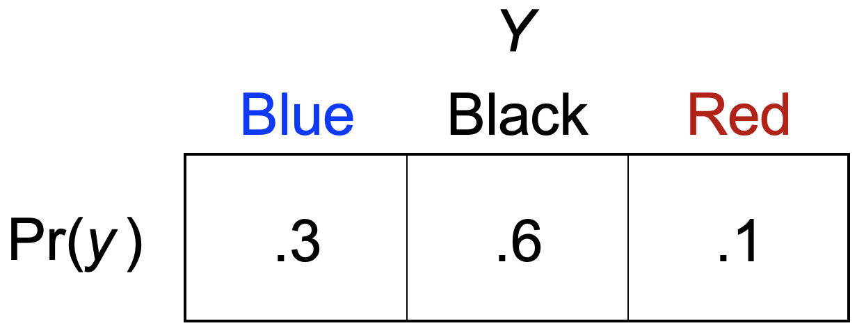
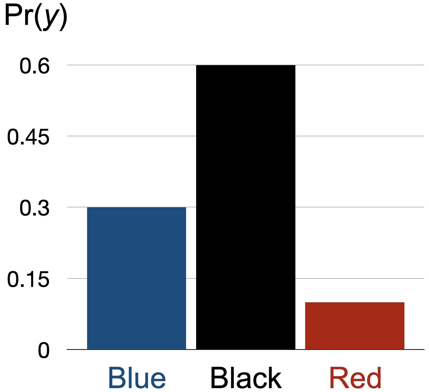
Consider one more example of a discrete distribution. Suppose we have a bag full of marbles. There are different numbers of Blue marbles, Black marbles, and Red marbles in the bag. If we shake the bag and pull out a marble, the PMF for the marble color is \[\begin{equation} \Pr(y)= \left\{ \begin{array}{ccl} .3 & \, & \mbox{if }\, y={\color{blue}{\mbox{Blue}}} \\ .6 && \mbox{if } \, y={{\mbox{Black}}} \\ .1 && \mbox{if } \, y={\color{red}{\mbox{Red}}} \end{array} \right. \tag{11.3} \end{equation}\] Again, a rough interpretation is that 30% of the time we will pull out a Blue marble, 60% of the time we will pull out a Black marble, and 10% of the time we will pull out a Red. Axioms 1 and 2 are satisfied: the probability of each outcome is non-negative and they all sum to one. The third axiom is built in, so it is satisifed as well – e.g., the probability of extracting either a Blue marble or a Red marble is \(\Pr({\color{blue}{\mbox{Blue}}} \, \mbox{or} \, {\color{red}{\mbox{Red}}} )=\Pr({\color{blue}{\mbox{Blue}}}) + \Pr({\color{red}{\mbox{Red}}} ) = .3 + .1 = .4\).
11.4.1 The Complement
A very useful result of the axioms is that we can make use of the complement to simplify some calculations. Consider the die toss and suppose we want to calculate the probability of not observing a 6 as the outcome. One way we could calculate that is to calculate \[\Pr(\mbox{not} \, 6) = \Pr(1) + \Pr(2) + \Pr(3) + \Pr(4) + \Pr(5) = \frac{1}{6} + \frac{1}{6} +\frac{1}{6} +\frac{1}{6} +\frac{1}{6} = \frac{5}{6}\] Given our outcomes in the die toss, the complement of the set \(\{1, 2, 3, 4, 5 \}\) is simply observing 6 as an outcome – it’s the only outcome left. We can therefore calculate the probability of not observing a 6 as \[\Pr(\mbox{not} \, 6) = 1- \Pr(6) = 1-\frac{1}{6} = \frac{5}{6}\]
Let’s apply the same concept to the bag of marbles. We can calculate the probability of drawing a Blue or Black marble as \[\Pr(\color{blue}{\mbox{Blue}} \, \mbox{or} \, \mbox{Black}) = \Pr({\color{blue}{\mbox{Blue}}}) + \Pr({\mbox{Black}} ) = .3 + .6 = .9\] or we can use the complement \[ \Pr(\color{blue}{\mbox{Blue}} \, \mbox{or} \, \mbox{Black}) = 1- \Pr({\color{red}{\mbox{Red}}}) = 1 -.1 = .9\]
11.5 PMFs as Equations, Tables, and Graphs
Throughout the rest of this course, we’ll see probability distributions displayed in different ways. It’s important that you understand these versions. We’ve already seen one common form of a PMF: an equation. For the marbles example, we wrote the PMF as \[\begin{equation} \Pr(y)= \left\{ \begin{array}{ccl} .3 & \, & \mbox{if }\, y={\color{blue}{\mbox{Blue}}} \\ .6 && \mbox{if } \, y={{\mbox{Black}}} \\ .1 && \mbox{if } \, y={\color{red}{\mbox{Red}}} \end{array} \right. \end{equation}\] Honestly, using an equation for the PMF in this case isn’t necessarily a simpler way to communicate that information. We’ll see later, however, that using equations for PMFs can convey a lot of information in a relatively efficient manner.
For something like the marbles PMF, it might make more sense to communicate the PMF as a table like the following:

Finally, we’ll sometimes express a probability distribution graphically.

11.6 Cumulative Probability
We have already seen that we can calculate the probability that one of multiple events will occur: we can use the last rule from the axioms of probability. A special case of that is to calculate the probability that our random variable is less than some value.
For an interval-scale random variable \(Y\), the cumulative probability that \(Y\) is less than or equal to some value \(y\) is \[\Pr(Y\le y) = \sum_{y_i \le y} \Pr(y_i)\]
Notice that we can’t apply this to an unordered, categorical variable. For our bag of marbles, it doesn’t make sense to ask what the probability is of picking a marble that is less than or equal to a Black marble.
Let’s take a look at a few examples of cumulative probability. However, instead of using our fair die’s PMF, we’ll assume that we have a “loaded die” with the following PMF:

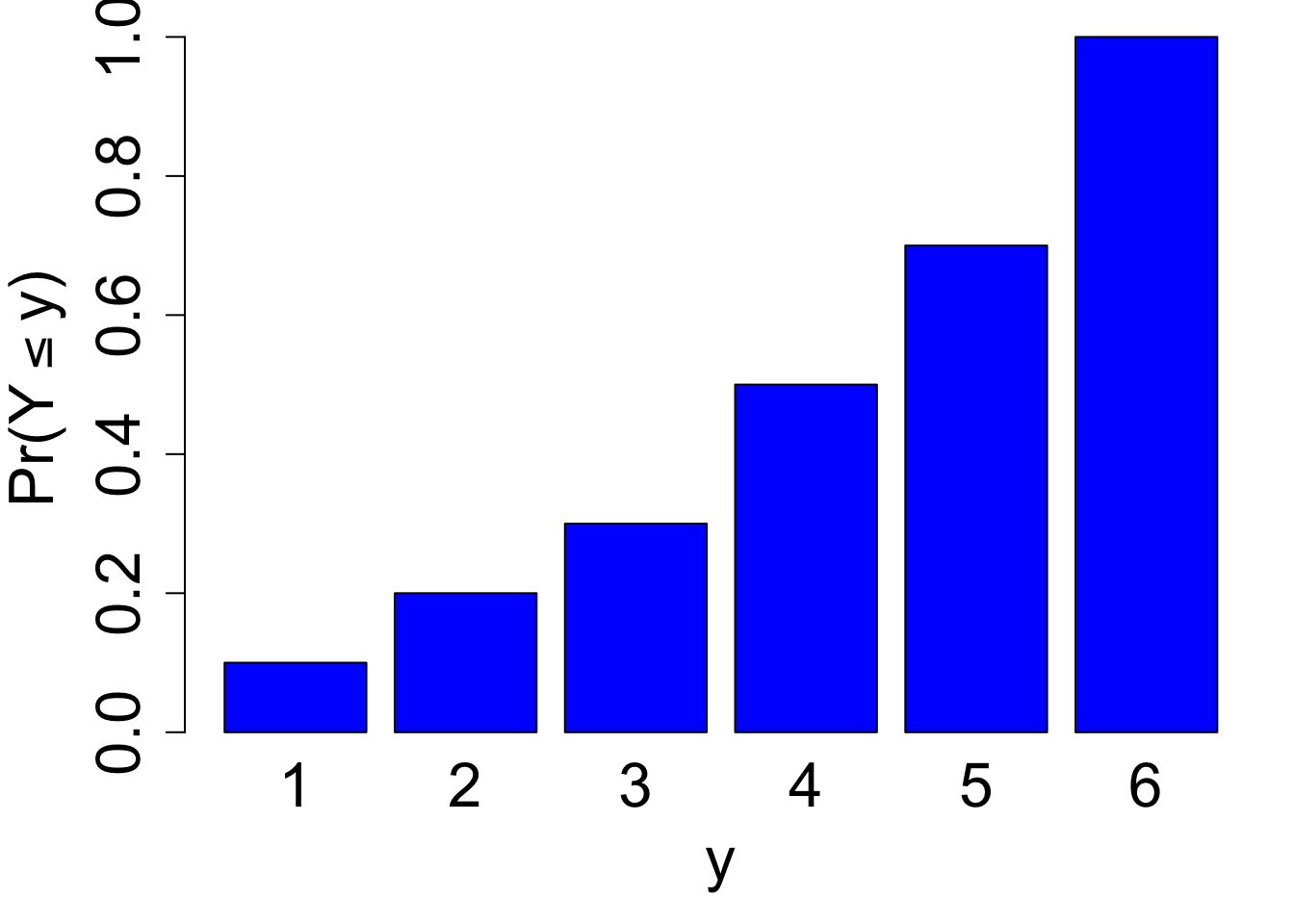
We can calculate the cumuluative probability for any value of \(y\) from one to six: \[\begin{align} \Pr(Y\le 1) &= \Pr(1) = .1\\ \Pr(Y\le 2) &= \Pr(1) + \Pr(2)= .1 + .1 = .2\\ \Pr(Y\le 3) &= \Pr(1) + \Pr(2) + \Pr(3) = .1 + .1 .+ 1 = .3\\ \Pr(Y\le 4) &= \Pr(1) + \Pr(2) + \Pr(3) + \Pr(4) = .1 + .1 + .1 + .2 = .5\\ \Pr(Y\le 5) &= \Pr(1) + \Pr(2) + \Pr(3) + \Pr(4) + \Pr(5) = .7\\ \Pr(Y\le 6) &= \Pr(1) + \Pr(2) + \Pr(3) + \Pr(4) + \Pr(5) + \Pr(6)= 1 \end{align}\]
The calculations we just made define \(Y\)’s cumulative distribution function (cdf). As we increase the value of the random variable, the cdf increases (or at least never decreases), moving towards a maximum value of one. We can plot the loaded die’s cdf

11.6.1 Variations on Cumulative Probability
There are many variations of the cumulative calculation. Again, we’ll use the loaded die PMF.

Strict versus Non-Strict Inequality
\[\begin{align} \Pr(Y<3) &= \Pr(1) + \Pr(2) = .1 + .1 = .2\\ \Pr(Y<6) &= \Pr(1) + \Pr(2) + \Pr(3) + \Pr(4) + \Pr(5) = .7 \end{align}\]
Greater Than
\[\begin{align} \Pr(Y\ge 5) &= \Pr(5) + \Pr(6) = .2 + .3 = .5\\ \Pr(Y>3) &= \Pr(4) + \Pr(5) + \Pr(6) = .2 + .2 + .3 = .7 \end{align}\]
Complement
\[\begin{align} \Pr(Y<6) &= 1-\Pr(6) = 1-.3 = .7\\ \Pr(Y>1) &= 1-\Pr(1) = 1-.1 = .9 \end{align}\]
Range of Values
\[\begin{align} \Pr(2\le Y \le 4) &= \Pr(2) + \Pr(3) + \Pr(4) = .1 + .1 + .2 = .4\\ \Pr(3 < Y \le 5) &= \Pr(4) + \Pr(5) = .2 + .2 = .4 \end{align}\]
Practice Session: Discrete Probability, Basic Calculations
The following is an interactive practice session. In the main panel, a probability mass function is displayed as a table. The possible outcomes are shown along the top and their probabilities are directly below. You are asked to calculate a probability, which you can do in R, with a calculator, or with pencil & paper. Enter your answer in the supplied box and click Submit. Hit Next to generate a new question. Try to solve at least five or six problems – more if you’re having difficulty with them.